Getting Started#
Important
The cemd package revolves around the
AtomicSystem class, which serves as the primary container for all atomic data: coordinates, topology, box parameters, masses, and force field parameters.
Creating a System#
Every example below works on the same system, so start by building one –
a 30 Å box of water at 1.0 g/cm³. Nothing has to be downloaded:
SolutionBuilder works out how many molecules the
target density calls for and packs them with Packmol.
from cemd.build import SolutionBuilder

system = SolutionBuilder.from_water(density=1.0).build(box=[30.0, 30.0, 30.0])
system.summary()
<AtomicSystem with 2709 atoms, 1806 bonds, 903 angles>

Box
 a (Å)  b (Å)  c (Å)  α (°)  β (°)  γ (°)
 30.00  30.00  30.00  90.00  90.00  90.00

Atoms
type  number      mass  charge
  Hw    1806  1.007947   0.446
  Ow     903 15.999430  -0.892

Bonds
 type  number
Hw-Ow    1806

Angles
    type  number
Hw-Ow-Hw     903

Total charge: 0.000 e
Volume: 27.00 nm³
Density: 1.00 g/cm³
The water already carries its force-field atom types (Ow, Hw) and
the SPC/E charges that go with them.
Loading a System#
An existing structure is read with
from_file(), which picks the
reader from the extension:
from cemd import AtomicSystem

system.write("waterbox.data")            # from the box built above
system = AtomicSystem.from_file("waterbox.data")
Supported for reading: .data and .lmp (LAMMPS), .cif, .pdb,
.sdf and .lt (moltemplate). Writing supports .data and .pdb.
Creating a System from SMILES#
You can also create molecules directly from their SMILES string:
# Create a simple molecule
ethanol = AtomicSystem.from_smiles("CCO")

# Create a more complex molecule
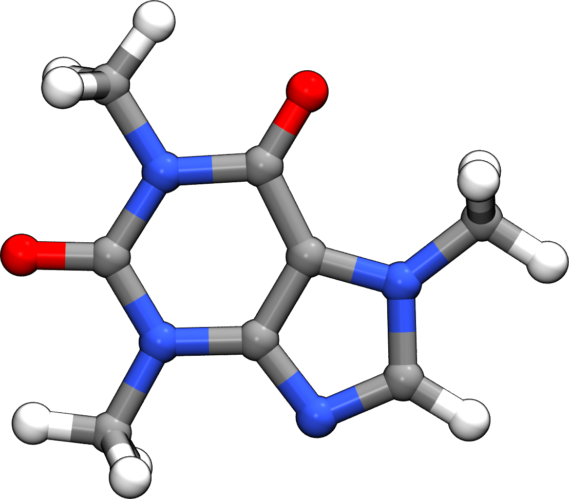
caffeine = AtomicSystem.from_smiles("CN1C=NC2=C1C(=O)N(C(=O)N2C)C")

# Visualize the molecule
caffeine.view()
Interactive Database Exploration#
CEMD provides interactive interfaces to explore and load structures from open databases.
Crystallography Open Database (COD)#
from cemd import AtomicSystem

# Launches an interactive TUI to browse COD
system = AtomicSystem.from_cod()
? Search by: (Use arrow keys)
» Mineral Name
  Chemical Formula
  COD ID
? Search by: Mineral Name
? Enter your query: calcite
Found 145 structures  [20/145]
↑↓ Move   [Enter] Load   [d] DOI   [w] COD page   [q] Quit

      ID | NAME                 | FORMULA            | LATTICE PARAMETERS                    | DOI
----------------------------------------------------------------------------------------------------
   1001741 | Nitrocalcite         | - Ca H8 N2 O10 -   |   6.3   9.2  14.9 |  90° 106°  90°    |  ✓
   1001743 | Nitrocalcite         | - Ca H8 N2 O10 -   |   6.3   9.1  14.8 |  90° 106°  90°    |  -
   1010917 | Barytocalcite        | - C2 Ba Ca O6 -    |   8.2   5.2   6.6 |  90° 106°  90°    |  -
➜  1010928 | Calcite              | - C Ca O3 -        |   6.4   6.4   6.4 |  46°  46°  46°    |  ✓
   1010962 | Calcite              | - C Ca O3 -        |   6.4   6.4   6.4 |  46°  46°  46°    |  -
   1011029 | Nitratine            | - N Na O3 -        |   6.3   6.3   6.3 |  47°  47°  47°    |  ✓
   1011228 | Rhodochrosite        | - C Mn O3 -        |   5.8   5.8   5.8 |  48°  48°  48°    |  ✓
   ...     | ...                  | ...                | ...                                       | ...

  ↕ 1-20 of 145
PubChem Database#
from cemd import AtomicSystem

# Interactive PubChem explorer
molecule = AtomicSystem.from_pubchem()
Inspecting a System#
Once loaded, the AtomicSystem object provides immediate access to physical
properties and topology:
# Basic properties
print(f"Box parameters [a, b, c, α, β, γ] : {system.box}")
print(f"Number of atoms : {system.num_atoms}")
print(f"Atom types      : {system.atom_types}")
print(f"Density         : {system.density:.3f} g/cm³")
print(f"Total charge    : {system.total_charge:.4f} e")
print(f"Volume          : {system.volume:.2f} ų")
Box parameters [a, b, c, α, β, γ] : [30 30 30 90 90 90]
Number of atoms : 2709
Atom types      : ['H', 'O']
Density         : 1.000 g/cm³
Total charge    : 0.0000 e
Volume          : 27000.00 ų
# Direct access to the atoms DataFrame
print(system.atoms.head(10))
      type  charge          x          y       z
id
1       O     0.0  14.507000  26.157000  14.212
2       H     0.0  13.987000  25.868000  13.408
3       H     0.0  15.459000  26.318001  13.954
4       O     0.0  16.625999  16.400000  13.285
5       H     0.0  15.970000  15.702000  12.997
6       H     0.0  17.561001  16.048000  13.139
7       O     0.0  25.382999  11.912000  19.295
8       H     0.0  24.693001  11.469000  18.738
9       H     0.0  26.286999  12.003000  18.814
10      O     0.0  17.439001   3.114000  14.050

[10 rows x 5 columns]
Counting Specific Atom Types#
# Count specific atom types
n_si = system.get_count("Si")
n_ca = system.get_count("Ca")
n_h2o = system.get_count("O") // 2  # Rough estimation for water

print(f"Si atoms: {n_si}, Ca atoms: {n_ca}, H2O molecules: {n_h2o}")
Manipulating Systems#
Adding Atoms#
# Add a single atom
system.add_atom("Na", [5.0, 5.0, 5.0], charge=1.0)

# Add multiple atoms at once
system.add_atoms(
    atypes=["Na", "Cl", "Na"],
    positions=[[0, 0, 0], [10, 0, 0], [20, 0, 0]],
    charges=[1.0, -1.0, 1.0]
)
Removing Atoms#
# Remove specific atoms by index
system.remove_atoms([1, 2, 3])

# Remove a single atom
system.remove_atom(5)
Setting Box Parameters#
# Set a cubic box
system.set_box([30, 30, 30, 90, 90, 90])

# Set an orthorhombic box
system.set_box([20, 30, 25, 90, 90, 90])
Replicating the System#
# Replicate the system 2x in x, 3x in y, 1x in z
system.replicate([2, 3, 1])
Wrapping Atoms (PBC)#
# Bring all atoms back into the box
system.wrap()

# Center the system on its center of mass
system.center_on_com()

# Center only specific atom types
system.center_on_com(atom_types=["Ca", "Si"])
Protonating Atoms#
# Protonate specific atoms
system.protonate_atoms([10, 15, 20], bond_length=1.0)

# Protonate a single atom
system.protonate_atom(10, bond_length=1.0)
Saving a System#
To write a system back to a LAMMPS .data file:
# Save with the default atom style (preserved from the input file)
system.write("output.data")

# Specify the atom style explicitly
system.write("output.data", atom_style="full")    # full: id mol type charge x y z
system.write("output.data", atom_style="charge")  # charge: id type charge x y z
Note
The .data format is the recommended output format for LAMMPS simulations.
The system can also be exported to the .pdb.
Converting a System#
To MDAnalysis#
Convert to a MDAnalysis Universe for advanced trajectory analysis:
u = system.to_mda()
print(u)
<Universe with 2709 atoms>

# Access trajectory frames
for ts in u.trajectory:
    print(ts.frame, ts.positions.shape)
To Pymatgen#
Convert to a Pymatgen Structure for crystallographic analysis:
struct = system.to_pmg()
print(struct)
Full Formula (H1806 O903)
Reduced Formula: H2O
abc   :  30.000000  30.000000  30.000000
angles:  90.000000  90.000000  90.000000
pbc   :       True       True       True
Sites (2709)
   #  SP            a          b          c    charge
----  ----  ---------  ---------  ---------  --------
   0  O      0.483567   0.8719     0.473733         0
   1  H      0.466233   0.862267   0.446933         0
   2  H      0.5153     0.877267   0.465133         0
   ...
Visualization#
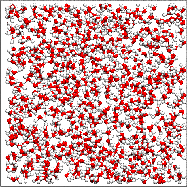
You can visualize your system in VMD directly from Python:
# Static view of the current configuration
system.view()

# View with an associated MD trajectory
system.view(trajectory="md_production.dcd")
Setting Force Fields#
From Database#
Load force field parameters from the built-in database:
# Map atom types to force field parameters
assignments = {
    'O': 'ospc',   # Water oxygen (SPC model)
    'H': 'hspc',   # Water hydrogen (SPC model)
    'Si': 'st',    # Tetrahedral silicon (ClayFF)
    'Ca': 'ca'     # Aqueous calcium (ClayFF)
}

# Apply the force field
system.set_ff_from_database(assignments)

# Interactive force field explorer
system.explore_ff_database()
Manual Assignment#
from cemd.forcefield.models import LJParams

# Set masses
system.set_masses({'H': 1.008, 'O': 15.999, 'Si': 28.085})

# Set charges
system.set_charges({'H': 0.41, 'O': -0.82, 'Si': 2.1})

# Set Lennard-Jones self-interaction parameters (epsilon, sigma)
system.set_pair_params('Si', params=LJParams(epsilon=0.000184, sigma=3.302))

# Apply mixing rules for cross-interactions (requires that every atom
# type already has a self-interaction LJ pair set, as above)
system.apply_pair_mixing_rules(rule='arithmetic')
Setting Topology#
Automatic Detection#
# Apply ClayFF topology rules
system.set_topology('clayff')

# Apply CSHFF topology rules (ClayFF + specific calcium handling)
system.set_topology('cshff')

# Automatically detect angles, dihedrals and impropers from bonds
system.guess_connections()
Custom Rules#
from cemd.topology import TopologyRule, NeighborCriterion

# Define a custom rule: an O bonded to exactly 2 H within 1.2 A becomes
# "Ow", its H neighbors become "Hw", and the O-H bonds/H-O-H angle are
# created.
custom_rule = TopologyRule(
    center="type O",
    neighbors=[NeighborCriterion("type H", cutoff=1.2, count=2, new_type="Hw")],
    new_type="Ow",
    bonds=True,
    angles=True,
)

# Apply the rule
system.set_topology(custom_rule)

# Several rules can be applied in one call, in order
system.set_topology([custom_rule, another_rule])
Manual Connectivity#
# Add a bond between atoms 1 and 2
system.add_bond([1, 2])

# Add an angle (atoms 1-2-3)
system.add_angle([1, 2, 3])

# Add a dihedral (atoms 1-2-3-4)
system.add_dihedral([1, 2, 3, 4])

# Remove all connections
system.remove_all_connections()

# Keep only specific connection types
system.keep_connection_types(
    bond_types=["H-O", "Si-O"],
    angle_types=["H-O-H"]
)
Combining Systems#
To stack one structure on top of another (e.g. a molecule on a surface),
see add_structure(),
add_liquid_layer() and
add_droplet(), described in the
build guide.
To open a gap inside an existing system (optionally filling it with a
solution), use Splitter:
from cemd.build import Splitter, SolutionBuilder

# Cut the system at z=15 A and open a 30 A gap there
split_system = Splitter(system, coordinate=15.0, axis='z', gap_size=30.0).split()

# Or fill the gap with a solution (fluent API)
blueprint = SolutionBuilder(density=1.0, counts={'Na': 10, 'Cl': 10})
filled_system = (
    Splitter(system, coordinate=15.0, axis='z', gap_size=30.0)
    .add_solution(blueprint, padding=2.0)
    .split()
)